Spectral clustering is a machine learning technique used to group similar data points. What makes it special is that it does not just look at distances between points, unlike some other methods, such as K-Means clustering, which do. Instead, it first builds a similarity graph that connects data points that are similar to each other.

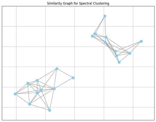
Imagine each data point as a dot, and if two dots are very alike, we draw a line between them. This web of connections forms what we call a similarity graph. From this graph, we can begin to understand the structure of the data, not just who is close to whom, but how the whole group is shaped. This ability enables spectral clustering to identify and group together clusters that are oddly shaped or complex, which other methods might overlook.

To analyze this similarity graph mathematically, we convert it into a matrix, a structured table of numbers, similar to a spreadsheet. Each row and column corresponds to a data point, and the numbers inside represent the strength of the connections between those points. From this matrix, we can calculate what is called the graph Laplacian, another matrix that reveals how the points are linked and how tightly clusters of them hold together. You don’t need to understand the exact mathematical details. Just think of it as measuring the “tension” within the network, showing how easily groups of points might separate from one another.

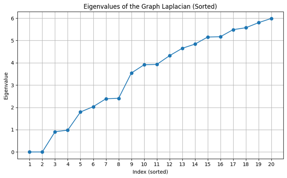
Once we have the Laplacian matrix, we can explore its hidden structure using two concepts from linear algebra: eigenvectors and eigenvalues. These tools help us simplify complex systems. You do not need to understand precisely how they work, but you can think of eigenvectors as special directions in space that don’t change direction when a transformation, such as stretching or rotating, is applied to them. Eigenvalues tell us how much those directions are stretched. In spectral clustering, we focus on the smallest eigenvalues and their corresponding eigenvectors because they reveal where the graph can be most naturally divided. It is similar to finding fault lines in a piece of rock—places where it naturally wants to break apart.

Once we’ve calculated these eigenvectors, we no longer use the original data. Instead, we cluster the numbers inside the eigenvectors. These numbers provide a new way to represent our data, one that makes the natural groupings much more apparent. So, spectral clustering isn’t just grouping things based on closeness; it’s transforming the data into a new form that reveals its actual structure, and then applying a simple clustering method, such as K-Means, to that transformed version.

If similarity graphs, matrices, eigenvalues, and eigenvectors seem complex, don’t worry. A deep mathematical background is not required to apply spectral clustering in practice. Modern tools like Python offer high-level implementations that significantly reduce the need for underlying computation. By continuing through this blog, you will see how spectral clustering can be executed efficiently and intuitively with just a few lines of code.

How It’s Used in Practice

Spectral clustering is a versatile tool used across various modern industries to enhance efficiency and productivity. In cybersecurity, it is especially effective for improving network intrusion detection, particularly in cases where attack instances are far less frequent than regular traffic. By capturing the underlying structure of the data, spectral clustering can significantly boost detection rates, making it valuable for identifying rare and complex attack patterns that traditional methods often miss.

In telecommunications, spectral clustering plays a key role in speaker diarization, which involves separating an audio recording by individual speakers. The process begins by extracting deep speaker embeddings and constructing an affinity graph that reflects the similarity between speech segments. Spectral clustering then effectively groups these segments, resulting in more accurate diarization, especially in complex acoustic environments. This approach often outperforms traditional clustering methods in precision.

Additionally, spectral clustering is used in medical imaging to segment and track lesions across multiple time points in 3D MRI scans, such as monitoring the progression of multiple sclerosis. Analyzing scans collectively rather than individually provides more robust and consistent lesion detection, ultimately improving diagnostic accuracy.

Putting It Together in Python

For this example, we will use a synthetic dataset that simulates employee behavior within a corporate network to detect insider threats. The dataset includes features such as average work hours, sensitive file accesses, email activity, failed login attempts, USB usage, after-hours actions, and VPN logins. It contains two distinct behavioral groups: normal users and insider threats who exhibit riskier activity patterns.

We will use Google Colab to run our code because it is easy to use while still offering powerful capabilities.

Step 1: Setup & Imports

First, we will import the required libraries. We need Pandas and NumPy for data handling, and StandardScaler for feature scaling, which is crucial for effective clustering. SpectralClustering will be used to perform the clustering itself, while PCA will help reduce the high-dimensional data to two dimensions, making visualization easier. Finally, matplotlib.pyplot will be used to plot and display the results.

import pandas as pd
import numpy as np
from sklearn.preprocessing import StandardScaler
from sklearn.cluster import SpectralCluster
from sklearn.decomposition import PCA
import matplotlib.pyplot as plt

Then, we’ll load the dataset. Copy the file path and paste it into the line of code.

df = pd.read_csv('**PASTE PATH HERE**')

After that, we’re going to remove the label column because this type of clustering is unsupervised, so we don’t use the labels directly during the clustering process.

X = df.drop(columns=['label'])

Step 2: Feature Scaling

Next, we’ll use StandardScaler to standardize the data. This means we will rescale each feature to have a mean of zero and a standard deviation of one. Standardizing is important because spectral clustering relies on distance and similarity calculations, and features measured on different scales (for example, hours versus file counts) could distort the results.

scaler = StandardScaler()
X_scaled = scaler.fit_transform(X)

Step 3: Apply Spectral Clustering

We will now apply spectral clustering to the dataset.

sc = SpectralClustering(n_clusters=2, affinity='rbf', gamma=1.0, random_state=42)
y_pred = sc.fit_predict(X_scaled)

Because the dataset has seven behavioral features, each point exists in a 7-dimensional space, which we cannot visualize directly. To make the data easier to plot, we will turn the 7-dimensional space into a two-dimensional representation.

pca = PCA(n_components=2)
X_pca = pca.fit_transform(X_scaled)
df_clustered = pd.DataFrame(X, columns=X.columns)
df_clustered['cluster'] = y_pred
cluster_means = df_clustered.groupby('cluster').mean()
insider_cluster = cluster_means['sensitive_file_accesses'].idxmax()
label_map = {insider_cluster: 'Insider Threats', 1 - insider_cluster: 'Normal Users'}

Step 4: Plotting and Annotation

Finally, we will plot the results and add labels to help visualize the clustered groups.

plt.figure(figsize=(8, 6))
scatter = plt.scatter(X_pca[:, 0], X_pca[:, 1], c=y_pred, cmap=’viridis’, s=80, edgecolor=’k’)
plt.title(‘Spectral Clustering on Insider Threat Dataset’)
plt.xlabel(‘PCA Component 1’)
plt.ylabel(‘PCA Component 2’)
plt.grid(True)
for cluster_id in [0, 1]:
cluster_points = X_pca[y_pred == cluster_id]
center = cluster_points.mean(axis=0)
plt.text(center[0], center[1], label_map[cluster_id],
fontsize=12, weight=’bold’, bbox=dict(facecolor=’white’, alpha=0.8),
ha=’center’, va=’center’)
plt.tight_layout()
plt.show()

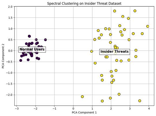
The final result should look like this: normal users on the left and insider threats on the right.

Auxin GitHub

The complete code is available on the Auxin GitHub repository.

Conclusion

Spectral clustering is a powerful and flexible technique that helps uncover hidden patterns in complex datasets, especially when those patterns do not follow simple shapes. By transforming data into a graph and analyzing its structure using tools from linear algebra, spectral clustering can produce more accurate and meaningful groupings than many traditional methods.

As shown through both the explanation and the Python demo, you do not need a deep mathematical background to apply this method effectively. Whether you are detecting insider threats in cybersecurity or segmenting lesions in medical imaging, spectral clustering provides a modern and practical solution for finding structure in data. It is a valuable tool worth exploring in any data science toolkit.