Mean Shift clustering is a machine learning algorithm used to group data points based on their density. Unlike K-Means clustering, it doesn’t require specifying the number of clusters in advance, as it automatically identifies cluster centers.

Mean Shift clustering works by first creating a circular window (akin to a search area) over each data point and calculating the average (mean) position of all nearby points within that window. Then, the window moves (or “shifts”) to this new average position. This process continues until the window stops moving, indicating it has reached a high-density area, or “peak.” All points that are pulled to the same peak are assigned to the same cluster.

The key setting in Mean Shift is the bandwidth, which controls the size of the search window. A smaller bandwidth finds more detailed clusters, while a larger one creates fewer, broader clusters. Mean Shift is beneficial when you don’t know how many clusters to expect and when the clusters aren’t neatly shaped.

Industry Use Cases

In cybersecurity, mean shift clustering has been applied to network anomaly detection and intrusion detection systems (IDS), especially in unsupervised settings where attack patterns are not known in advance. For instance, in SCADA systems that monitor industrial infrastructure, mean-shift has been used to pre-cluster sensor data and network traffic, helping isolate unusual behavior indicative of attacks. Its strength lies in its ability to dynamically group similar behaviors without prior knowledge, making it ideal for detecting novel or stealthy threats in dynamic environments, such as operational networks and IoT systems.

Outside of cybersecurity, mean-shift has been widely used in remote sensing and computer vision. In hyperspectral image segmentation, it enables the unsupervised classification of land cover types by clustering superpixels based on both spectral and spatial features, offering accurate results without the need for labeled training data. In forestry and urban planning, 3D lidar data are processed using mean shift clustering to delineate individual trees from complex point clouds automatically. Meanwhile, in robotics and computer vision, the mean shift algorithm is used in object segmentation pipelines, where deep pixel embeddings are clustered to identify unseen object instances, enabling autonomous systems to detect and interact with unfamiliar objects. Across these domains, the mean-shift algorithm’s ability to adapt to data structure without requiring manual tuning of cluster numbers makes it a robust tool for real-world applications involving noisy, high-dimensional, or unlabeled datasets.

A Closer Look at the Math

Mean Shift clustering is a technique that groups data points by locating the areas where points are most concentrated, using a method based on kernel density estimation.

This is the formula for kernel density estimation:

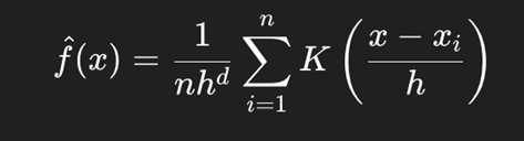
The variable n Is the total number of data points in the dataset? The term h Is the bandwidth. d Represents the number of dimensions in the data, adjusting for the volume of the kernel in a multi-dimensional space. Inside the summation, Σ, each xi Is an individual datapoint from the dataset, and the expression measures the scaled distance between the estimation point x and each datapoint xi. The Kernel function K then assigns a weight to that distance: points closer to x Contribute more to the estimate, while farther ones contribute less. The Kernel function can be many different functions, such as the Epanechikov or Uniform function, but it will most likely be a radial basis function (RBF kernel) in this case. The sum over all n Points accumulate these weighted contributions to give a smooth estimate of density at x.

The RBF kernel formula is this:

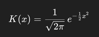
In essence, the KDE formula calculates the number of points near x, their closeness, and the weight each should be given, all while scaling appropriately for the data’s dimensions.

The result is a weighted average, and the algorithm moves the point in the direction of that average. This movement, known as the mean shift vector, is recalculated and applied repeatedly until the point stops moving significantly, meaning it has reached a high-density area, or mode. Once all points have converged to their respective modes, points that arrive at the same or nearby locations are grouped into the same cluster.

While the underlying mathematics may appear complex, Python can simplify the process by performing all the necessary calculations for you.

Step-by-Step Python Example

We will be using Google Colab due to its powerful capabilities and user-friendly interface, making it an ideal choice for beginners.

For this demonstration, we’ll use a dataset that captures different user behavior patterns within a system. Each row represents a user and includes two key metrics: the number of login attempts per hour and the average session duration. These behavioral patterns can reveal distinctions between regular users, administrators, bots, and potentially suspicious activity. This makes the dataset ideal for exploring how clustering algorithms, like Mean Shift, can be used to group similar users based on their activity.

System Setup

import pandas as pd
import matplotlib.pyplot as plt
from sklearn.cluster import MeanShift, estimate_bandwidth
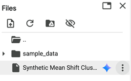
import numpy as np

Next, import your CSV file into Google Colab. Once uploaded, copy the file path and paste it into the following line of code to read the file.

df = pd.read_csv(" **PASTE PATH HERE** ")

Preparing the Input Data

We will then select the two numerical features that the clustering algorithm will use to identify patterns in the data.

X = df[["Login Attempts/hr", "Avg Session Duration (min)"]].values

Then, we’ll compute an appropriate bandwidth value, which specifies how close data points must be to be grouped within the same cluster.

bandwidth = estimate_bandwidth(X, quantile=0.2, n_samples=400)

Executing the Mean Shift Algorithm

Next, we’ll apply the mean shift clustering

ms = MeanShift(bandwidth=bandwidth, bin_seeding=True)
ms.fit(X)
labels = ms.labels_
cluster_centers = ms.cluster_centers_
n_clusters = len(np.unique(labels))

Visualizing the Results

Then, we will assign labels to each cluster and visualize the results using a scatter plot. To enhance clarity, we will also plot the cluster centers.

df["Cluster"] = labels
plt.figure(figsize=(8, 6))
for k in range(n_clusters):
cluster = df[df["Cluster"] == k]
plt.scatter(cluster["Login Attempts/hr"], cluster["Avg Session Duration (min)"], label=f'Cluster {k}')
plt.scatter(cluster_centers[:, 0], cluster_centers[:, 1], 
c='black', s=200, marker='x', label='Centers')
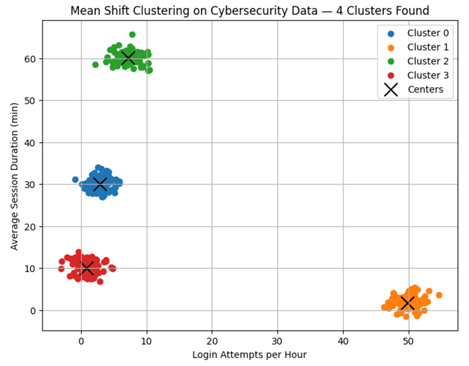
plt.title(f'Mean Shift Clustering on Cybersecurity Data — {n_clusters} Clusters Found')
plt.xlabel("Login Attempts per Hour")
plt.ylabel("Average Session Duration (min)")
plt.legend()
plt.grid(True)
plt.show()

The result should look like this.

Auxin Github

You can download this full notebook at our Auxin GitHub.

Insights and Observations

Mean Shift Clustering provides a powerful and flexible approach to discovering patterns in unlabeled data, eliminating the need to predefine the number of clusters. Its mathematical foundation in kernel density estimation enables it to adapt to complex data shapes and densities, making it particularly useful in domains such as cybersecurity, computer vision, and remote sensing.

As demonstrated in the Python example, implementing this algorithm can be straightforward and highly effective, even for beginners. Whether you’re analyzing network traffic or segmenting images, Mean Shift provides a dynamic tool for uncovering hidden structure in your data.