What is Hierarchical Clustering?

Hierarchical clustering is a machine learning method that groups things based on likeness. Imagine this: You have a group of animals, and you want to categorize them based on their similarities. Cats and tigers go together. Eagles and pigeons go together. Then you can group all the birds and all the cats. Eventually, you build a tree showing how all the animals are related to each other. That tree is called a dendrogram.

A dendrogram is a visual representation of hierarchical clustering that looks like a branching tree. It shows how individual data points or objects are grouped step-by-step, starting with each point as its cluster at the bottom and gradually merging similar clusters as you move up. The vertical height of each branch indicates the degree of similarity or difference between the merged clusters (the lower the branch, the more similar the items are).  Dendrograms are a helpful way to understand the relationships and structure within data, showing both broad groupings and finer subclusters in one clear diagram.

Practical Use Cases of Hierarchical Clustering

Hierarchical clustering is widely used across various modern industries to uncover natural groupings within complex data, enabling more informed and targeted decisions. In retail and e-commerce, companies analyze customer purchase histories and demographics using hierarchical clustering to create detailed customer segments. This approach enables businesses to tailor marketing campaigns and promotions to specific groups, such as budget-conscious shoppers or loyal brand buyers, ultimately driving higher sales and enhancing customer engagement.

Similarly, in healthcare, hierarchical clustering can group patients based on their medical records and disease profiles, allowing providers to identify high-risk subgroups or distinct types of cancer. These insights support personalized treatment plans and targeted interventions, which have been shown to improve patient outcomes and reduce hospital readmissions.

Financial institutions also leverage hierarchical clustering to enhance portfolio management and risk assessment. By grouping stocks or clients based on characteristics like sector, volatility, or credit behavior, firms can build diversified investment portfolios and identify risk segments more effectively. This reduces overall portfolio risk and enables banks to customize interest rates or monitoring for different customer clusters.

In transportation, hierarchical clustering helps planners analyze traffic patterns by grouping road segments with similar congestion or usage profiles. This hierarchical view enables targeted traffic management strategies, such as adjusting signal timings or prioritizing infrastructure upgrades, which optimize flow and reduce bottlenecks.

For telecommunications, hierarchical clustering is used to optimize both network resources and customer retention efforts. Operators cluster cell towers by load patterns to decide where to increase capacity and segment subscribers by usage to tailor retention campaigns.

In cybersecurity, hierarchical clustering plays a critical role in anomaly detection and threat identification. By grouping devices, users, or network events based on configuration or behavior, security teams can spot outliers that may indicate compromised systems or malicious activity. The hierarchical nature of the clustering provides a visual map that allows for zooming in on suspicious clusters, enabling the detection of novel threats that evade traditional security rules.

Across these industries, hierarchical clustering transforms raw data into actionable insights by revealing meaningful patterns and relationships at multiple levels of detail.

The Math Behind It

Hierarchical clustering begins with calculating the distance between data points. Three commonly used distance metrics are Euclidean distance, Manhattan distance, and maximum distance. Euclidean distance measures the straight-line distance between two points in space and is calculated as the square root of the sum of squared differences across all features or dimensions. Manhattan distance, sometimes called city-block distance, sums the absolute differences across each dimension, resembling the distance you’d travel navigating a grid of city streets. The maximum distance (or Chebyshev distance) considers only the most considerable absolute difference in any one dimension, effectively measuring the most significant step required along any coordinate axis.

Once all pairwise distances between data points are computed, hierarchical clustering treats each point as an individual cluster and starts merging the closest clusters. Determining which clusters are closest depends on the linkage method. Four popular linkage criteria are single linkage, complete linkage, average linkage, and Ward linkage. Single linkage uses the minimum distance between any two points in the two clusters, merging clusters based on their closest members. This often produces elongated, chain-like clusters because clusters can be connected through close individual points.

At each step of the clustering process, the distances between clusters are updated based on the chosen linkage criterion, and the two clusters with the smallest inter-cluster distance merge. This process continues until all points are grouped into a single large cluster. The dendrogram visually records these merging steps, where the height of each branch corresponds to the distance at which clusters were combined.

This process may seem tedious, but in the modern day, we have tools that can automate it for us. In this blog, you’ll be walked through how to make your hierarchical cluster using a Jupyter-style notebook, Google Colab.

Setting Up

Google Colab is a powerful yet beginner-friendly platform for working with Python. Today, we’ll use a realistic synthetic dataset containing fruit samples, each described by attributes such as weight (in grams), sweetness level, color intensity, and genus (a categorical label).

Before we begin to code, we need to import some libraries. The imports bring in tools to handle data tables (pandas), scale features (sklearn.preprocessing), perform hierarchical clustering and plot dendrograms (scipy.cluster.hierarchy), and create visualizations (matplotlib.pyplot).

import pandas as pd
import numpy as np
from sklearn.preprocessing import StandardScaler
import matplotlib.pyplot as plt
from scipy.cluster.hierarchy import dendrogram, linkage, fcluster

Next, we’ll import our dataset.

# Load dataset
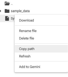
df = pd.read_csv(‘ **PASTE THE PATH OF YOUR FILE HERE** ’)

Initializing our Inputs

After that, we’ll begin the actual coding. The numeric columns (weight, sweetness, and color intensity) are selected separately, as clustering algorithms require numerical input.

# Numeric features
num_features = df[['weight_grams', 'sweetness_level', 'color_intensity']]

Meanwhile, the categorical genus feature must be converted into a numerical form so it can influence the clustering process.

# One-hot encode genus
genus_dummies = pd.get_dummies(df['genus'])

Incorporating Genus into Hierarchical Clustering

To incorporate genus information, the code utilizes one-hot encoding, which transforms the categorical genus labels into binary columns —one for each unique genus. For example, if there are five genera, the encoding creates five columns where each fruit has a 1 in the column corresponding to its genus and 0s elsewhere. This numeric representation allows clustering algorithms to consider genus as part of the feature space.

However, since the numeric features and the genus features have different scales and meanings, the numeric features are standardized using feature scaling. This scaling normalizes the numeric features to have a mean of zero and a standard deviation of one, preventing features with larger ranges from dominating the distance calculations.

# Scale numeric features
scaler = StandardScaler()
num_scaled = scaler.fit_transform(num_features)

After scaling, we’ll make the genus features more heavily weighted by multiplying their values by a factor (in this example, 3). This step ensures that genus differences have a more substantial impact on the clustering outcome, effectively telling the algorithm to prioritize grouping fruits by genus alongside their numeric similarity. Next, the scaled numeric features and the weighted genus features are combined into a single feature matrix. This combined matrix is then used to compute hierarchical clusters using the Ward linkage method, which aims to minimize variance within clusters.

# Weight genus features more strongly by multiplying
genus_weight = 3  # try 3 or higher to emphasize genus
genus_weighted = genus_dummies.values * genus_weight
# Combine scaled numeric and weighted genus features
features = np.hstack([num_scaled, genus_weighted])

Plotting the Dendrogram

Finally, we’ll visualize the hierarchical clustering result by plotting a dendrogram using the dendrogram function.

# Plot dendrogram with fruit names
plt.figure(figsize=(12, 6))
dendrogram(
    linked,
    labels=df['fruit_name'].values,
    orientation='top',
    distance_sort='ascending',
    show_leaf_counts=True,
    leaf_rotation=90
)
plt.title('Hierarchical Clustering of Fruit Samples')
plt.xlabel('Fruit Name')
plt.ylabel('Distance')
plt.tight_layout()
plt.show()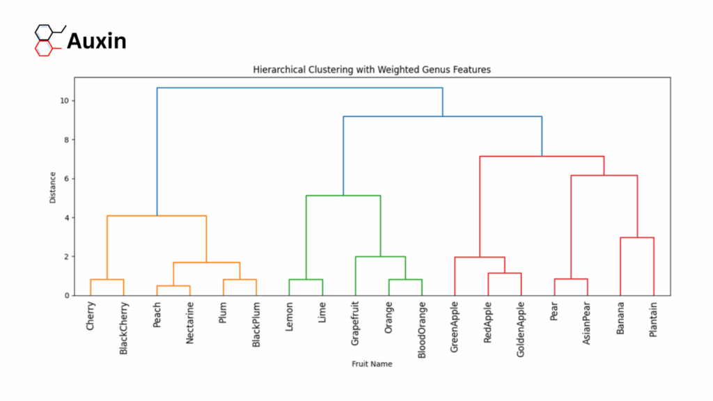

As you can see, the samples are clustered according to their genus, then by the similarity of their physical features.

Auxin Github

You can download this full notebook at our Auxin Github.

Key Takeaways

Hierarchical clustering is a powerful, intuitive method for uncovering natural groupings in complex datasets, offering both visual clarity through dendrograms and practical insights across a wide range of industries. From customer segmentation and medical diagnostics to financial analysis and cybersecurity, its ability to reveal multi-level relationships makes it an essential tool for modern data analysis.

By understanding the underlying mathematics and experimenting with real data in Python, even beginners can harness this technique to make more informed, data-driven decisions. With accessible tools like Google Colab and open-source libraries, hierarchical clustering is now more approachable than ever.