SVM? What’s That?
The Support Vector Machine (SVM) is a machine learning technique used to find the boundary between two distinct classes. It attempts to draw a line (called a hyperplane) that distinguishes between the two classes. SVM will look for the line that best separates the different classes, maximizing the distance between the line and the nearest points from both sides. The distance between the nearest points is referred to as the margin, and the data points that are the closest to the hyperplane are called the support vectors.

How It’s Used
SVMs have numerous applications across various industries. For example, in healthcare, SVMs are used to detect cancer from medical scans like MRIs. They learn the difference between images of healthy and cancerous tissue, which can help doctors make faster and more accurate diagnoses. In finance, banks utilize SVMs to predict whether an individual is likely to default on a loan. By examining factors such as income, credit history, and other personal information, the SVM can determine if someone is a high-risk borrower.
In cybersecurity, SVMs help spot hackers or unusual activity on a network. They learn what regular internet traffic looks like and flag anything strange as a possible attack.

In factories, SVMs are used for predictive maintenance. They analyze machine sensor data to predict when a component is likely to fail, enabling timely repairs before a costly breakdown occurs. Finally, in image recognition, SVMs excel at recognizing handwritten numbers and letters, such as converting pictures of digits into actual numbers for sorting mail or filling out digital forms. These examples demonstrate how SVMs are applied in everyday technology to address real-world problems.
The Kernel Trick
When the data is not linearly separable in its original space, meaning you can’t draw a straight line (or hyperplane) to divide the classes, the kernel trick is used. Imagine trying to classify two groups of dots on a graph: blue dots in the middle, and red dots surrounding them in a ring. No matter how you try, you can’t draw a straight line that separates the two groups.

This is referred to as a non-linearly separable problem. A basic SVM, which draws a straight line or plane to split the data, would struggle here.
This is where the kernel trick comes in. Instead of trying to separate the data in its current form (say, in two dimensions), the idea is to transform the data into a higher dimension where it becomes easier to separate. For example, you can add a third feature to each point based on its distance from the center of the graph. This lifts the data into 3D, and now the previously inseparable points can be cleanly separated by a flat plane. The transformation makes the problem solvable in a new environment.
However, doing all these calculations in a higher dimension can be complicated and slow. The kernel trick solves this by avoiding the transformation altogether. Instead, it uses a special function called a kernel that calculates the same result, as if the data had been mapped to a higher dimension, without actually doing the mapping. This shortcut allows SVMs to handle complex patterns and curved boundaries with the speed and simplicity of working in the original space.
The math behind the kernel trick involves using a kernel function 𝐾 (𝑥, 𝑥 ′ ) to compute the inner product of two points after they’ve been transformed into a higher-dimensional space by a mapping function 𝜙. Instead of explicitly calculating 𝜙(𝑥) and 𝜙(𝑥 ′ ) and then their dot product 𝜙 (𝑥 ) ⋅ 𝜙 (𝑥 ′ ), the kernel function directly computes this value using the original inputs:

One common variant is the polynomial kernel, which measures similarity between two points using their dot product raised to a power.

Another is the RBF (Radial Basis Function) kernel, which excels at drawing curved boundaries between classes.
These kernel functions enable SVMs to learn complex decision surfaces, such as circles or spirals, without requiring the heavy lifting of higher-dimensional math. That’s the power of the kernel trick: it lets simple algorithms solve complex problems by thinking in higher dimensions, without ever going there.
If the formulas look intimidating to you, don’t worry. This blog will guide you through running an SVM, in just five minutes, using Google Colab, which will do the calculations for you.
Data Collection
First, we need to import some libraries. NumPy is a Python library used for numerical computing. It provides powerful tools for working with arrays, performing mathematical operations, and efficiently handling large datasets. We need Matplotlib for the visualizations and Scikit-learn for its machine learning operations. Additionally, we’ll need to upload the dataset we’ll be using.
import matplotlib.pyplot as plt
from sklearn import svm, datasets
import numpy as np
Next, we need to initialize the dataset we will use. For this example, we will use the Iris dataset, a small, classic dataset commonly used in machine learning. It contains 150 samples of iris flowers from three species: Setosa, Versicolor, and Virginica. Each sample has four features: sepal length, sepal width, petal length, and petal width, which are all measured in centimeters. The goal is to predict the species based on these measurements.
With this technology, scientists can develop a lightweight, convenient mobile tool that utilizes measurements of petals, which are easily measurable in the field, to classify iris species quickly.
‘X’ will be the input features, petal length and petal width, and ‘y assigns the species labels (0, 1, or 2 for Setosa, Versicolor, Virginica).
iris = datasets.load_iris()
X = iris.data[:, 2:4]
y = iris.target
Training the Model
This code will create an SVM model that utilizes the RBF kernel, enabling it to learn non-linear boundaries.
Model = svm.SVC(kernel='rbf', C=1.0, gamma='auto')
model.fit(X, y)
Creating a Grid to Visualize the Decision Boundaries
Next, we need to define the area to plot the graph. To do this, we will find the minimum and maximum values of the petal length and width.
x_min, x_max = X[:, 0].min() - 0.5, X[:, 0].max() + 0.5
y_min, y_max = X[:, 1].min() - 0.5, X[:, 1].max() + 0.5
Then, we’ll create a grid of points across the plotting area, which we’ll classify to visualize the decision regions.
xx, yy = np.meshgrid(np.linspace(x_min, x_max, 500),
np.linspace(y_min, y_max, 500))
Plotting the Decision Boundaries and Data
Finally, we will plot the SVM data. As you can see, it’s accurate, primarily, except for a few points. This is because the Iris dataset is not perfectly separable by petal length and width alone. To make it accurate, you would need more data points. This is very common in the real world, as real data is often messy and features frequently overlap between classes, contain noise, or exhibit outliers.
Z = model.predict(np.c_[xx.ravel(), yy.ravel()])
Z = Z.reshape(xx.shape)
plt.contourf(xx, yy, Z, alpha=0.3, cmap=plt.cm.coolwarm)
plt.scatter(X[:, 0], X[:, 1], c=y, cmap=plt.cm.coolwarm, edgecolors='k')
plt.xlabel("Petal Length (cm)")
plt.ylabel("Petal Width (cm)")
plt.title("SVM Classification of Iris Species")
plt.show()

If you want labels for the different species, add this code before plt.xlabel(“Petal Length (cm)”).
species_names = iris.target_names
for i, species in enumerate(species_names):
    x_text = X[y == i, 0].mean()
    y_text = X[y == i, 1].mean()
    plt.text(x_text, y_text, species, fontsize=12, weight='bold',
    horizontalalignment='center', verticalalignment='center',
    bbox=dict(facecolor='white', alpha=0.6, edgecolor='black'))
Another Example
Here’s another example of an SVM in Python. It utilizes a realistic synthetic dataset comprising 20 sessions, each represented by five features: session duration, bytes sent, packets per second, whether a login attempt was made, and the number of failed connection attempts. Each session is labeled as 0 (benign) or 1 (malicious) based on suspicious behavior patterns, such as a high number of failed connections or speedy packet rates.
To make the model interpretable and visual, only two of the five features —packets per second and failed connections — are selected for classification and visualization. These features are then scaled using StandardScaler so that the SVM isn’t biased toward any one feature due to differences in units or range. An SVM with an RBF kernel is trained on this scaled 2D data. This kernel enables the model to draw nonlinear decision boundaries, thereby improving its ability to separate complex patterns between malicious and benign behavior.
The next step involves creating a mesh grid that covers the feature space. The trained SVM model predicts the class for every point in this grid, and those predictions are used to plot decision regions. Finally, a contour plot is generated to display these regions, along with the original session points colored by class (red for malicious and blue for benign). This visualization clearly shows how the SVM draws boundaries between safe and risky traffic based on behavioral traits, illustrating how AI can be used for real-time threat detection in cybersecurity environments.

Here, malicious sessions are marked in red, while benign sessions are marked in blue.
Complete Code at the Auxin GitHub
You can download the code for the cyber sessions SVM, as well as the Iris SVM, from our Auxin GitHub.
To Wrap Things Up
Support Vector Machines (SVMs) are powerful and versatile tools for classification and regression tasks. By finding the optimal boundary that separates data into distinct classes, SVMs aim to maximize accuracy and generalization.
Their ability to handle both linear and non-linear problems, especially with the help of kernel functions, makes them suitable for a wide range of real-world applications, from image recognition to medical diagnosis. While they may require careful tuning and computational resources for large datasets, SVMs remain a reliable choice for tasks where high precision and clear margins are essential.