
This simple tutorial, written by Auxin Security’s engineers Adam Khalil and Ekin Yilmaz, helps learn logistic regression and create a model in Jupyter Notebook in just five minutes. Logistic Regressions are a powerful yet simple machine learning method used to examine the probability of a dependent variable (for example, yes/no, true/false, success/failure) based on one or more predictor variables. It is one of the simplest regression analysis methods for predicting the probability of an event. This technique is called logistic regression because it uses a logistic function to transform a linear regression into a probability.
What is Logistic Regression, and How is it Used?
Logistic regressions have many real-world applications. For instance, healthcare professionals can predict the likelihood of a person developing a disease based on their age, lifestyle, and genetics. In cybersecurity, logistic regressions can be used to sort and detect malware by analyzing file size, file origin, and behavior. It can also be used to detect various cyberattacks, such as phishing emails and ATO (account takeover). The technique accomplishes this by analyzing behavior, such as changes in email or new login locations. The following examples illustrate how logistic regressions help identify trends and aid in classification problems.
Platforms such as Auxin AI streamline the use of advanced statistical modeling by offering secure and intuitive solutions that enable developers to build AI applications efficiently while safeguarding their data. It also facilitates tasks such as regression analysis by allowing different AI tools to work together seamlessly, which saves time and money.
To have a clearer understanding of logistic regressions, consider the case of the likelihood that a website visitor clicks the checkout button on your website. Logistic regression analysis uses past data, such as the time spent on the website and the number of items in the cart, to make a prediction. It determines that, in the past, if visitors spent more than five minutes on the site and added more than three items to the cart, they clicked the checkout button. Using this information, the logistic regression function can then predict the behavior of a new website visitor.
The mathematical equation, called a sigmoid function, of a logistic regression is given by:
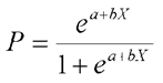
Here, P represents the probability of the dependent variable being 1 (e.g., success, pass) for the given independent variable X. e is the base of the natural logarithm. A is the intercept, which is the log-odds of P=1 when X=0, and b is the slope of the independent variable X, describing the change in the log-odds for a one-unit increase in X. The coefficients a and b are hypothetical model parameters estimated from the data. Their size determines the precision with which the model forecasts outcomes. The coefficients are estimated using mechanisms such as maximum likelihood estimation, whereby the values that make observed data most likely are computed.
Implementing Logistic Regression in Python
We will use a dataset to demonstrate the application of logistic regression analysis. Specifically, we’ll be working with hypothetical data on student study and sleep habits, which contains information on whether a student slept well and how many hours they studied for a test.
Setting up your system
Skip installing Python and use the Online Jupyter Platform
Google Colab will be the machine learning model we use. Google Colab, short for Google Colaboratory, is a free, cloud-based platform that lets you write and execute Python code in a Jupyter notebook environment.
It’s easy to use for beginners and well-suited for machine learning tasks, offering access to powerful computing resources, including GPUs and TPUs. This makes it an excellent option for machine learning projects. Let’s begin by adding the application to Google Drive.

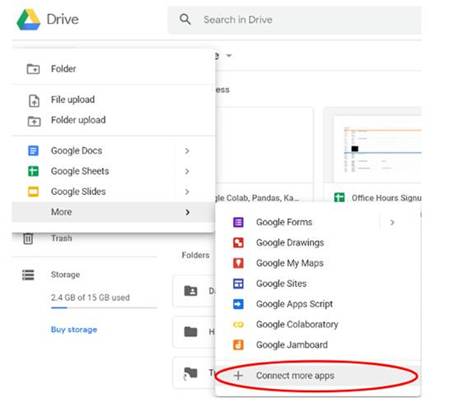
Open Drive and select the New button. In the dropdown menu, select Connect more apps (if you don’t already have Google Colab enabled), search for Colab, and add it to your Drive.
Finally, create a new Colab notebook by clicking the new button and finding it in the “More” drop-down menu. That’s it. We’re all set up and ready to get started.
Data Collection
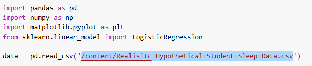
First, we need to import some libraries. We need Pandas for data manipulation, NumPy for mathematical calculations, and Matplotlib for visualizations. Sklearn libraries are used for machine learning operations.
Import pandas as pd
import numpy as np
import matplotlib.pyplot as plt
from sklearn.linear_model import LogisticRegression
Loading the Dataset
Next, download the dataset you want to use to make the Logistic Regression. Here, we’re using a hypothetical data set that measures how long students studied, whether they slept well the night before a test, and whether they passed the test. We will load the dataset and read it into a Pandas data frame.
data = pd.read_csv('/content/Realisitc Hypothetical Student Sleep Data.csv')Ensure that the contents of the parentheses match your file path. You can verify this by clicking on the three dots next to the file, then selecting ‘Copy path’ and pasting it into the parentheses.
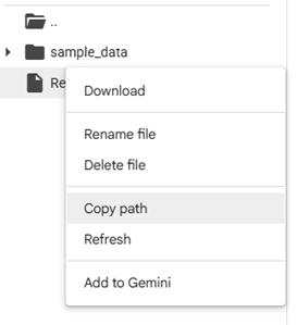
Make sure you have quotations surrounding the path as well.
Prepare the Features and Labels
We need to initialize what we want to use to make predictions and what we want the model to predict. X are the inputs, and Y is the output/target.
X = data[['Hours_Studied', 'Slept_Well']].values
y = data['Passed'].values
Training the Logistic Regression Model
Now, we create the logistic regression model and train it using our input and output values ‘X’ and ‘y
model = LogisticRegression()
model.fit(X, y)
Predicting Passing Probabilities
After training, the model can estimate the likelihood that a student will pass based on the hours studied and their sleep patterns. We provide new test data where the hours studied change, but the student always slept well. The model then calculates a probability between 0 and 1, indicating the likelihood of passing for each case. These probabilities enable us to determine how likely passing is as study time increases, provided adequate sleep is obtained.
hours = np.linspace(0, 7, 100)
sleep = np.ones_like(hours)  # slept well = 1
X_test = np.column_stack((hours, sleep))
prob_pass = model.predict_proba(X_test)[:, 1]
Plotting the Data
Finally, we’ll create a graph using a sigmoid function to display the results. The curve on the graph represents the model’s predicted probability of passing for different amounts of hours studied when the student slept well. We also plot the original data points, allowing you to see the actual examples used to train the model, with colors indicating whether the student slept well or not. This visual helps us understand how the predicted chance of passing changes with study time and sleep.
plt.figure(figsize=(8, 5))
plt.plot(hours, prob_pass, label='Predicted Probability of Passing', color='blue')
plt.scatter(data['Hours_Studied'], data['Passed'], c=data['Slept_Well'], cmap='coolwarm', edgecolors='k', label='Training Data')
plt.xlabel('Hours Studied')
plt.ylabel('Probability of Passing')
plt.title('Predicted Probability of Passing vs. Hours Studied (Assuming Good Sleep)')
plt.grid(True)
plt.legend()
plt.show()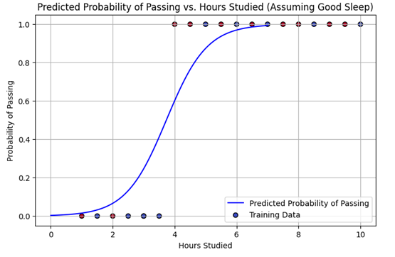
Full Code at the Auxin GitHub
You can download the entire code and the notebook from our Auxin GitHub.
Let’s Sum Up
Logistic regression is a powerful tool for predicting simple outcomes by modeling the relationship between variables. We demonstrated how this method can effectively estimate the probability of an event occurring, such as predicting whether an applicant will be admitted to a program based on their test scores or how the number of hours spent studying relates to the chance of passing.
We implemented this equation in Python to visualize and validate these predictions, highlighting the model’s efficiency in real-world applications. To improve scalability and security in AI-driven applications, platforms like Auxin AI provide low-code solutions that simplify development while protecting data integrity.